Customize The Plot
CustomizeThePlot.RmdIntroduction
An important feature of ggcoverage is the support of customization. This vignette will show how to customize the plot from the following two aspects:
- customize the elements of existing plot
- add additional layer to the existing plot
Customize the theme
Inner object
Before we start, let me introduce the internal structure of layers provided by ggcoverage. ggcoverage provides twelve layers, and geom_coverage, geom_protein are based solely on ggplot2, while the others are based on ggplot2 and patchwork.
| Modules | Type | Description | Object |
|---|---|---|---|
| geom_coverage | Coverage | Create genome coverage plot | ggplot2 |
| geom_base | Annotation | Add base, base frequency and amino acid annotations | ggplot2, patchwork |
| geom_cnv | Annotation | Add CNV annotation | ggplot2, patchwork |
| geom_gc | Annotation | Add GC content annotation | ggplot2, patchwork |
| geom_gene | Annotation | Add gene annotation | ggplot2, patchwork |
| geom_transcript | Annotation | Add gene’s transcripts annotation | ggplot2, patchwork |
| geom_peak | Annotation | Add peak annotation | ggplot2, patchwork |
| geom_ideogram | Annotation | Add chromosome ideogram annotation | ggplot2, patchwork |
| geom_tad | Annotation | Add contact map annotation | ggplot2, patchwork |
| geom_link | Annotation | Add link annotation | ggplot2, patchwork |
| geom_protein | Coverage | Create protein coverage plot | ggplot2 |
| geom_feature | Annotation | Add feature annotation for genome/protein coverage | ggplot2, patchwork |
By the way, all inner themes used are available in theme_ggcoverage.R
Library
# library
library(ggplot2)
library(patchwork)
library(tidyverse)
library(ggcoverage)
library(rtracklayer)
Prepare data
# prepare gtf
gtf.file = system.file("extdata", "used_hg19.gtf", package = "ggcoverage")
gtf.gr = rtracklayer::import.gff(con = gtf.file, format = 'gtf')

# sample metadata
sample.meta = data.frame(SampleName=c('Chr18_MCF7_ER_1','Chr18_MCF7_ER_2','Chr18_MCF7_ER_3','Chr18_MCF7_input'),
                         Type = c("MCF7_ER_1","MCF7_ER_2","MCF7_ER_3","MCF7_input"),
                         Group = c("IP", "IP", "IP", "Input"))
sample.meta
## SampleName Type Group
## 1 Chr18_MCF7_ER_1 MCF7_ER_1 IP
## 2 Chr18_MCF7_ER_2 MCF7_ER_2 IP
## 3 Chr18_MCF7_ER_3 MCF7_ER_3 IP
## 4 Chr18_MCF7_input MCF7_input Input
# track folder
track.folder = system.file("extdata", "ChIP-seq", package = "ggcoverage")
# load bigwig file
track.df = LoadTrackFile(track.folder = track.folder, format = "bw", region = "chr18:76822285-76900000",
                         meta.info = sample.meta)
# check data
head(track.df)
## seqnames start end score Type Group
## 1 chr18 76820285 76820400 219.658 MCF7_ER_1 IP
## 2 chr18 76820401 76820700 0.000 MCF7_ER_1 IP
## 3 chr18 76820701 76821000 439.316 MCF7_ER_1 IP
## 4 chr18 76821001 76821300 219.658 MCF7_ER_1 IP
## 5 chr18 76821301 76821600 0.000 MCF7_ER_1 IP
## 6 chr18 76821601 76821900 219.658 MCF7_ER_1 IP
track.df = track.df %>% dplyr::filter(Type %in% c("MCF7_ER_1", "MCF7_input"))
# create mark region
mark.region=data.frame(start=c(76822533),
                       end=c(76823743),
                       label=c("Promoter"))
# check data
mark.region
## start end label
## 1 76822533 76823743 Promoter
# create basic coverage plot
basic.coverage = ggcoverage(data = track.df, color = "auto", range.position = "out",
                            mark.region=mark.region, show.mark.label = FALSE)
basic.coverage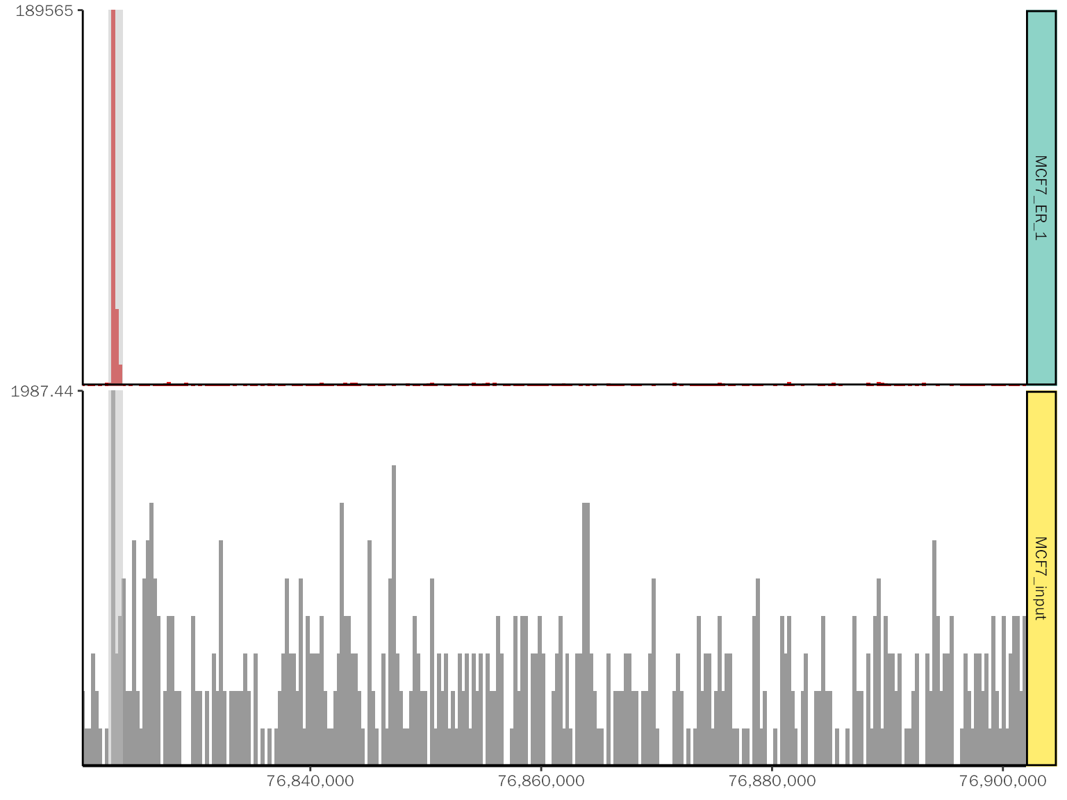
Customize ggplot2 object
Customize the plot generated by ggcoverage:
basic.coverage +
  # add title
  labs(title = "chr18:76,822,285-76,900,000") +
  theme(plot.title=element_text(hjust=0.5)) +
  # change color
  scale_fill_manual(values = c("MCF7_ER_1"="green", "MCF7_input"="yellow")) +
  # add rect
  geom_rect(
      data = data.frame(start = 76840533, end = 76842533),
      aes_string(xmin = "start", xmax = "end", ymin = "0", ymax = "Inf"),
      fill = "red", alpha = 0.6
    )
## Scale for fill is already present.
## Adding another scale for fill, which will replace the existing scale.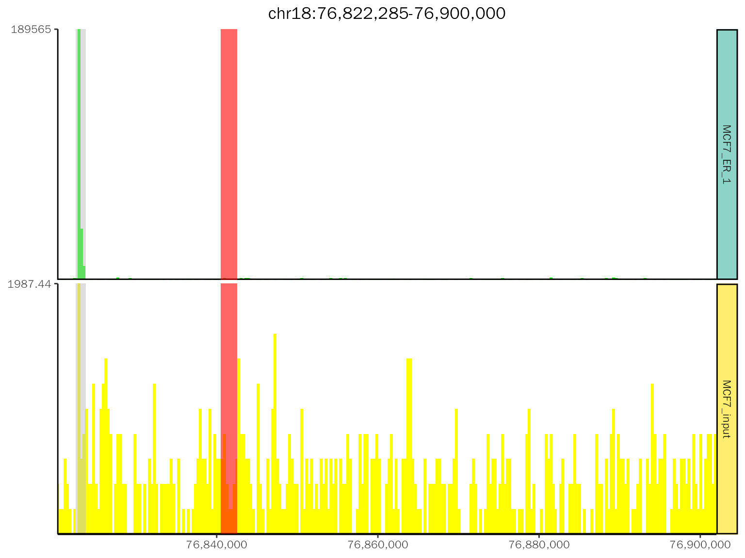
Customize patchwork object
patchwork is a ggplot2 extension, which is used to combine separate ggplots into the same graphic.
The example plot:
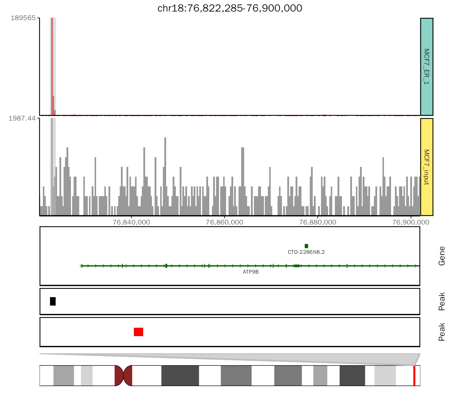
# get consensus peak file
peak.file = system.file("extdata", "ChIP-seq", "consensus.peak", package = "ggcoverage")
# example plot
chip.coverage = basic.coverage + labs(title = "chr18:76,822,285-76,900,000") +
  theme(plot.title=element_text(hjust=0.5)) +
  geom_gene(gtf.gr=gtf.gr, arrow.length = 0.04,arrow.size=0.25,
            gene.size = 0.75,
            utr.size = 1.5,
            exon.size = 2.5,label.size = 2.5, plot.height = 0.3) +
  geom_peak(bed.file = peak.file, plot.height = 0.1) +
  geom_ideogram(genome = "hg19",plot.space = 0, plot.height = 0.15)
## Loading ideogram...## Loading ranges...## Scale for x is already present.
## Adding another scale for x, which will replace the existing scale.
# get the class of chip.coverage
class(chip.coverage)
## [1] "patchwork" "gg" "ggplot"
# output the plot
chip.coverage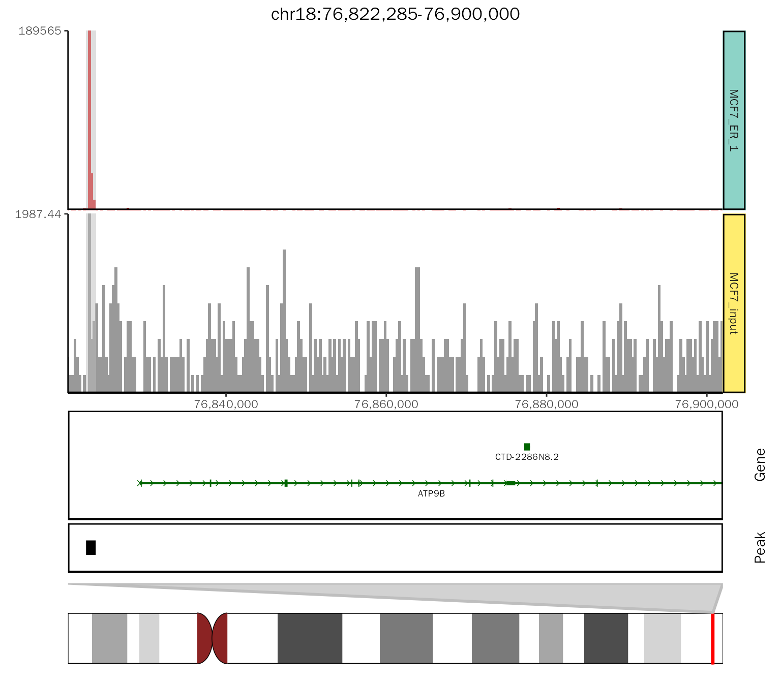
The above plot is a nested combination of ggplot2 object. We can obtain the elements (Pay attention to changes in object):
# obtain the track other than ideogram
chip.coverage[[1]]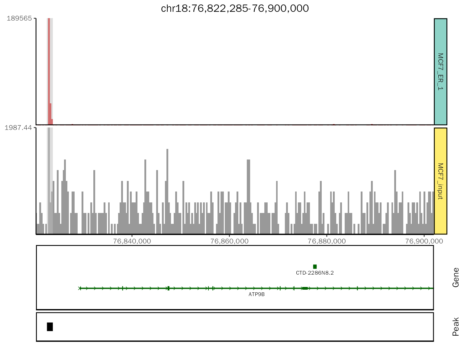
# class
class(chip.coverage[[1]])
## [1] "patchwork" "gg" "ggplot"
# obtain the track other than peak
chip.coverage[[1]][[1]]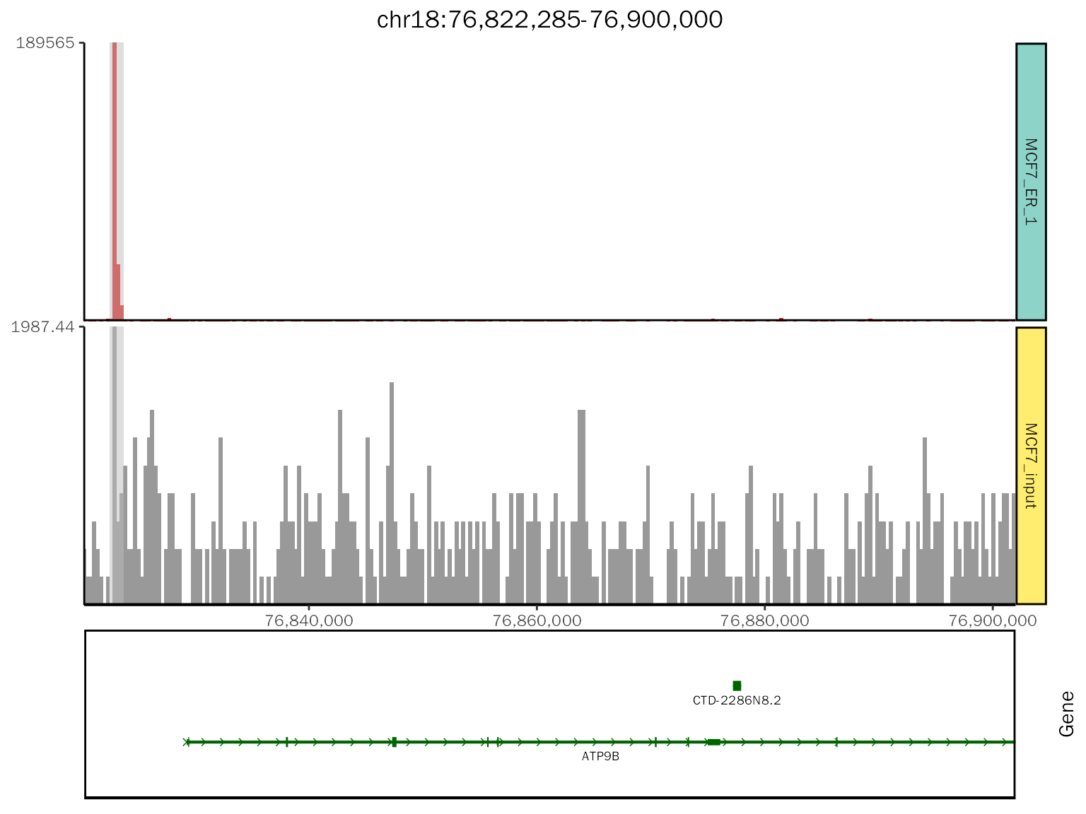
# class
class(chip.coverage[[1]][[1]])
## [1] "patchwork" "gg" "ggplot"
# obtain the gene track
chip.coverage[[1]][[1]][[2]]
# class
class(chip.coverage[[1]][[1]][[2]])
## [1] "gg" "ggplot"
# obtain the peak track
chip.coverage[[1]][[2]]
# class
class(chip.coverage[[1]][[2]])
## [1] "gg" "ggplot"Add another peak info:
chip.coverage[[1]][[2]] +
  # the size is the height of segment, controlled by peak.size in geom_peak
  geom_segment(
      data = data.frame(start = 76840533, end = 76842533),
      aes_string(x = "start", xend = "end", y = "1", yend = "1"),
      color = "red", size = 5
    )
Add additional layer
Obtain the data
To add additional layer, we need to obtain the raw coverage data (for consistency). ggcoverage provides GetPlotData to obtain the data used to plot.
# get coverage data, the layer number is four
coverage.data = GetPlotData(plot = chip.coverage, layer.num = 4)
# inspect data
head(coverage.data)
## seqnames start end score Type Group
## 1 chr18 76820285 76820400 219.658 MCF7_ER_1 IP
## 2 chr18 76820401 76820700 0.000 MCF7_ER_1 IP
## 3 chr18 76820701 76821000 439.316 MCF7_ER_1 IP
## 4 chr18 76821001 76821300 219.658 MCF7_ER_1 IP
## 5 chr18 76821301 76821600 0.000 MCF7_ER_1 IP
## 6 chr18 76821601 76821900 219.658 MCF7_ER_1 IP
str(coverage.data)## 'data.frame': 431 obs. of 6 variables:
## $ seqnames: Factor w/ 1 level "chr18": 1 1 1 1 1 1 1 1 1 1 ...
## $ start : int 76820285 76820401 76820701 76821001 76821301 76821601 76821901 76822201 76822801 76823101 ...
## $ end : int 76820400 76820700 76821000 76821300 76821600 76821900 76822200 76822800 76823100 76823400 ...
## $ score : num 220 0 439 220 0 ...
## $ Type : Factor w/ 2 levels "MCF7_ER_1","MCF7_input": 1 1 1 1 1 1 1 1 1 1 ...
## $ Group : chr "IP" "IP" "IP" "IP" ...Add layer
Here, I will create a new peak layer as an example (this is a sample example that does not depend on the raw data, but when you use your own data, you should use the raw data as region constraint).
# create pseudo-peak, you can load your peak file instead (be aware of 0-based/1-based)
pseudo_peak = data.frame(chr="chr18", start = 76840533, end = 76842533)
# get region constraint
plot.region.start <- coverage.data[1, "start"]
plot.region.end <- coverage.data[nrow(coverage.data), "end"]

# create plot
peak.plot = ggplot() +
  geom_segment(
      data = pseudo_peak,
      aes_string(x = "start", xend = "end", y = "1", yend = "1"),
      color = "red", size = 5
    ) +
  labs(y="Peak") +
  theme_peak(margin.len = 0.1, x.range = c(plot.region.start, plot.region.end))
peak.plot
Combine the plot:
# add peak layer
add.peak = patchwork::wrap_plots(chip.coverage[[1]] + theme(plot.margin = margin(t = 0.1, b = 0.1)),
    peak.plot,
    ncol = 1, heights = c(1, 0.1)
  )
add.peak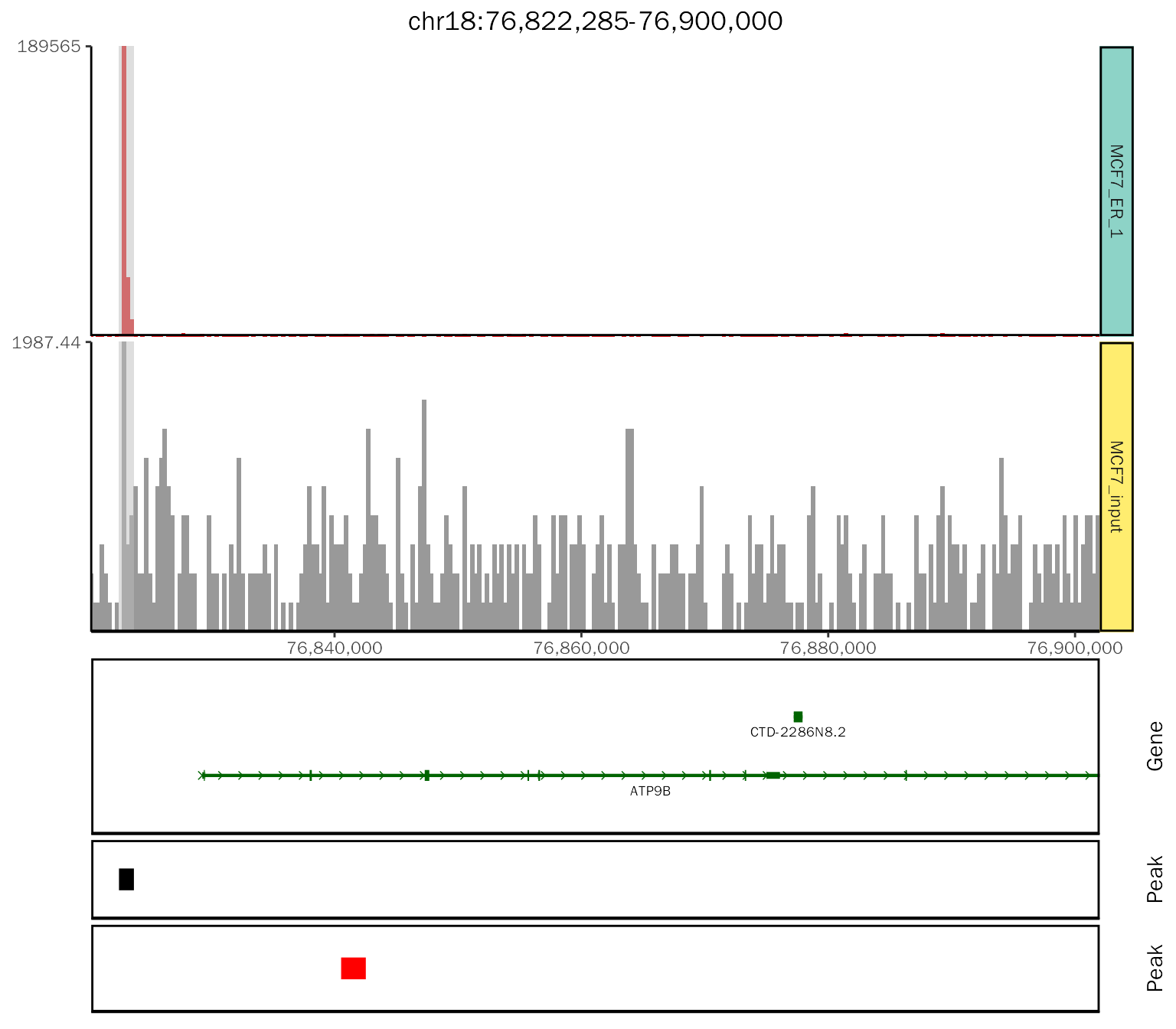
# add ideogram layers
final.plot = patchwork::wrap_plots(add.peak + theme(plot.margin = margin(t = 0.1, b = 0.1)),
    chip.coverage[[2]],
    ncol = 1, heights = c(1, 0.1)
  )
final.plot